介数

本示例演示了如何使用自定义调色板来可视化顶点介数和边介数。我们分别使用方法 igraph.GraphBase.betweenness() 和 igraph.GraphBase.edge_betweenness()，并演示其在标准 克拉卡特风筝图 以及一个 沃茨-斯特罗加茨 随机图上的效果。

import random
import matplotlib.pyplot as plt
from matplotlib.cm import ScalarMappable
from matplotlib.colors import LinearSegmentedColormap, Normalize
import igraph as ig

我们定义了一个函数，用于在 Matplotlib 轴上绘制图，并显示其顶点和边介数值。该函数还在两侧生成了一些颜色条，以显示它们之间的对应关系。我们使用 Matplotlib 的 Normalize 类 来确保颜色条范围正确，以及 igraph 的 igraph.utils.rescale() 将介数值重缩放到区间 [0, 1]。

def plot_betweenness(g, vertex_betweenness, edge_betweenness, ax, cax1, cax2):
    '''Plot vertex/edge betweenness, with colorbars

    Args:
        g: the graph to plot.
        ax: the Axes for the graph
        cax1: the Axes for the vertex betweenness colorbar
        cax2: the Axes for the edge betweenness colorbar
    '''

    # Rescale betweenness to be between 0.0 and 1.0
    scaled_vertex_betweenness = ig.rescale(vertex_betweenness, clamp=True)
    scaled_edge_betweenness = ig.rescale(edge_betweenness, clamp=True)
    print(f"vertices: {min(vertex_betweenness)} - {max(vertex_betweenness)}")
    print(f"edges: {min(edge_betweenness)} - {max(edge_betweenness)}")

    # Define mappings betweenness -> color
    cmap1 = LinearSegmentedColormap.from_list("vertex_cmap", ["pink", "indigo"])
    cmap2 = LinearSegmentedColormap.from_list("edge_cmap", ["lightblue", "midnightblue"])

    # Plot graph
    g.vs["color"] = [cmap1(betweenness) for betweenness in scaled_vertex_betweenness]
    g.vs["size"]  = ig.rescale(vertex_betweenness, (10, 50))
    g.es["color"] = [cmap2(betweenness) for betweenness in scaled_edge_betweenness]
    g.es["width"] = ig.rescale(edge_betweenness, (0.5, 1.0))
    ig.plot(
        g,
        target=ax,
        layout="fruchterman_reingold",
        vertex_frame_width=0.2,
    )

    # Color bars
    norm1 = ScalarMappable(norm=Normalize(0, max(vertex_betweenness)), cmap=cmap1)
    norm2 = ScalarMappable(norm=Normalize(0, max(edge_betweenness)), cmap=cmap2)
    plt.colorbar(norm1, cax=cax1, orientation="horizontal", label='Vertex Betweenness')
    plt.colorbar(norm2, cax=cax2, orientation="horizontal", label='Edge Betweenness')

首先，生成一个图，例如克拉卡特风筝图

random.seed(0)
g1 = ig.Graph.Famous("Krackhardt_Kite")

然后我们可以计算顶点和边介数

vertex_betweenness1 = g1.betweenness()
edge_betweenness1 = g1.edge_betweenness()

g2 = ig.Graph.Watts_Strogatz(dim=1, size=150, nei=2, p=0.1)
vertex_betweenness2 = g2.betweenness()
edge_betweenness2 = g2.edge_betweenness()

最后，我们绘制了这两个图，每个图都带有两个用于顶点/边介数的颜色条

fig, axs = plt.subplots(
    3, 2,
    figsize=(7, 6),
    gridspec_kw={"height_ratios": (20, 1, 1)},
)
plot_betweenness(g1, vertex_betweenness1, edge_betweenness1, *axs[:, 0])
plot_betweenness(g2, vertex_betweenness2, edge_betweenness2, *axs[:, 1])
fig.tight_layout(h_pad=1)
plt.show()

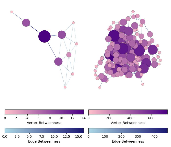
vertices: 0.0 - 14.0
edges: 1.5 - 16.0
vertices: 0.0 - 753.8235063912693
edges: 8.951984126984126 - 477.30745059034535