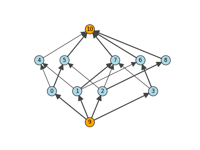
通过最大流实现最大二分图匹配

本例展示了如何使用最大流可视化二分图匹配（请参阅 igraph.Graph.maxflow()）。

注意

igraph.Graph.maximum_bipartite_matching() 通常是找到最大二分图匹配的更好方法。如需了解如何使用该方法，请参阅最大二分图匹配。

import igraph as ig
import matplotlib.pyplot as plt

我们首先创建二分有向图。

g = ig.Graph(
    9,
    [(0, 4), (0, 5), (1, 4), (1, 6), (1, 7), (2, 5), (2, 7), (2, 8), (3, 6), (3, 7)],
    directed=True
)

我们分配

• 节点0-3到一侧

• 节点4-8到另一侧

g.vs[range(4)]["type"] = True
g.vs[range(4, 9)]["type"] = False

然后我们添加一个源点（顶点9）和一个汇点（顶点10）

g.add_vertices(2)
g.add_edges([(9, 0), (9, 1), (9, 2), (9, 3)])  # connect source to one side
g.add_edges([(4, 10), (5, 10), (6, 10), (7, 10), (8, 10)])  # ... and sinks to the other

flow = g.maxflow(9, 10)
print("Size of maximum matching (maxflow) is:", flow.value)

Size of maximum matching (maxflow) is: 4.0

让我们将输出与 igraph.Graph.maximum_bipartite_matching() 进行比较

# delete the source and sink, which are unneeded for this function.
g2 = g.copy()
g2.delete_vertices([9, 10])
matching = g2.maximum_bipartite_matching()
matching_size = sum(1 for i in range(4) if matching.is_matched(i))
print("Size of maximum matching (maximum_bipartite_matching) is:", matching_size)

Size of maximum matching (maximum_bipartite_matching) is: 4

最后，我们可以很好地显示带有匹配项的原始流图。为了获得良好的视觉效果，我们手动设置源点和汇点的位置。

layout = g.layout_bipartite()
layout[9] = (2, -1)
layout[10] = (2, 2)

fig, ax = plt.subplots()
ig.plot(
    g,
    target=ax,
    layout=layout,
    vertex_size=30,
    vertex_label=range(g.vcount()),
    vertex_color=["lightblue" if i < 9 else "orange" for i in range(11)],
    edge_width=[1.0 + flow.flow[i] for i in range(g.ecount())]
)
plt.show()